Models

MLP

The Multi-Layer Perceptron (MLP) is a fully connected feedforward neural network. In XANESNET, it consists of an input layer, one or more hidden layers defined by num_hidden_layers, and an output layer. Each hidden layer is composed of a linear (dense) layer, a dropout layer for regularization, and an activation function. The output layer is a linear layer.

The size of the hidden layers is controlled by an initial hidden size hidden_size and a shrink rate shrink_rate, which multiplicatively reduces the number of neurons in successive hidden layers.

Input file:

• type: mlp

• params:

  • hidden_size (int, 512): Size of the first hidden layer.

  • dropout (float, 0.2): Dropout probability for hidden layers.

  • num_hidden_layers (int, 5): Number of hidden layers.

  • shrink_rate (float, 0.5): Multiplicative reduction factor for hidden layers.

  • activation (str, prelu): Activation function. Supported options: ReLU, Sigmoid, Tanh, PReLU, ELU, LeakyReLU, SELU, SiLU, GELU.

• weights (dict, optional): Configuration of the model weight initialisation, see model.

Example:

model:
  type: mlp
  params:
    hidden_size: 512
    dropout: 0.2
    num_hidden_layers: 5
    shrink_rate: 0.5
    activation: prelu
  weights:
    kernel: xavier_uniform
    bias: zeros
    seed: 2025

CNN

The Convolutional Neural Network (CNN) is a feedforward neural network commonly used for feature extraction from sequential or grid-like data. In XANESNET, the CNN consists of one or more 1D convolutional layers, followed by two fully connected (dense) hidden layers and an output layer for prediction.

Each convolutional layer contains a 1D convolution, batch normalization, an activation function, and dropout for regularization. The number of output channels for the first convolutional layer is defined by out_channel, and subsequent layers increase the number of channels multiplicatively by the factor channel_mul.

The first dense layer consists of a linear layer, a dropout layer, and activation function. The second dense layer consists of a linear layer only (output layer).

Input file:

• type: cnn

• params:

  • hidden_size (int, 256): Size of the initial hidden layer.

  • dropout (float, 0.2): Dropout probability for hidden layers.

  • num_conv_layers (int, 3): Number of convolutional layers.

  • out_channel (int, 32): Number of output channels for the initial convolutional layer.

  • channel_mul (int, 2): Channel multiplication factor for increasing output channels in subsequent convolutional layers.

  • kernel_size (int, 3): Size of the convolutional kernel.

  • stride (int, 1): Stride of the convolution operation.

  • activation (str, prelu): Activation function. Supported options: ReLU, Sigmoid, Tanh, PReLU, ELU, LeakyReLU, SELU, SiLU, GELU.

• weights (dict, optional): Configuration of the model weight initialisation, see model.

Example:

model:
  type: cnn
  params:
      hidden_size: 64
      dropout: 0.2
      num_conv_layers: 3
      activation: prelu
      out_channel: 32
      channel_mul: 2
      kernel_size: 3
      stride: 1
  weights:
    kernel: xavier_uniform
    bias: zeros
    seed: 2025

GNN

The Graph Neural Network (GNN) is a type of neural network that operates on graph-structured data. In XANESNET, the GNN processes node-level features using a sequence of customisable graph convolution layers (e.g., GCN, GAT, GATv2, GraphConv). Each layer includes batch normalization, activation, and dropout. These layers aggregate node features based on graph connectivity and edge attributes.

After the GNN layers, node-level embeddings are pooled using global mean pooling to produce a graph-level representation. This representation is then concatenated with additional global graph attributes (descriptor features) and passed through a final MLP to produce predictions.

Input file:

• type: gnn

• params:

  • layer_name (str, GATv2): Type of graph convolution layer. Options: GCN, GAT, GATv2, GraphConv.

  • layer_params (dict, optional): Parameters for the GNN layers.

  • hidden_size (int, 512): Size of hidden GNN layers.

  • dropout (float, 0.2): Dropout probability for GNN and MLP layers.

  • num_hidden_layers (int, 5): Number of GNN layers.

  • num_mlp_hidden_layers (int, 3): Number of hidden layers in the MLP.

  • activation (str, prelu): Activation function. Supported options: ReLU, Sigmoid, Tanh, PReLU, ELU, LeakyReLU, SELU, SiLU, GELU.

• weights (dict, optional): Configuration of the model weight initialisation, see model.

Example:

model:
    type: gnn
    params:
        layer_name: GATv2
        hidden_size: 512
        dropout: 0.2
        num_hidden_layers: 5
        num_mlp_hidden_layers: 3
        activation: prelu
        layer_params:
            heads: 2
            concat: True
            edge_dim: 16
    weights:
        kernel: xavier_uniform
        bias: zeros
        seed: 2025

LSTM

The Long Short-Term Memory (LSTM) network is a recurrent neural network to capture long-term dependencies in sequential data. In XANESNET, the LSTM model consists of a bidirectional LSTM layer, followed by two fully connected (dense) hidden layers.

The bidirectional LSTM layer processes the input sequence in both forward and backward directions. The output of the LSTM has a feature dimension of 2 x hidden_size. The first dense layer has size hidden_out_size. The second dense layer is the final output layer.

Input file:

• type: lstm

• params:

  • hidden_size (int, 256): Number of hidden units in the LSTM layer.

  • hidden_out_size (float, 128): Size of the intermediate dense layer after LSTM.

  • num_layers (int, 5): Number of LSTM layers.

  • dropout (float, 0.2): Dropout probability for the dense layers.

  • activation (str, prelu): Activation function. Supported options: ReLU, Sigmoid, Tanh, PReLU, ELU, LeakyReLU, SELU, SiLU, GELU.

• weights (dict, optional): Configuration of the model weight initialisation, see model.

Example:

model:
   type: lstm
   params:
     hidden_size: 256
     hidden_out_size: 128
     num_layers: 3
     dropout: 0.2
     activation: prelu
  weights:
    kernel: xavier_uniform
    bias: zeros
    seed: 2025

Transformer

The Transformer model in XANESNET implements a dual attention architecture to predict XANES spectra by modeling the interactions between local atomic environments and energy-dependent features.

The self-attention mechanism projects MACE features into a latent space defined by hidden_size. These embeddings undergo multiple rounds of self-attention via n_self_attn_layers to capture long-range structural dependencies between atoms in the system.

The cross-attention mechanism maps between the structural geometry and the energy domain. A learnable energy embedding is combined with additional features (e.g., PDOS) to provide a starting point for the cross-attention layers. By iterating through n_cross_attn_layers, the energy queries selectively extract structural information to determines the contributes of each atom to the absorption cross-section at a specific energy level. Final predictions are generated by passing the attended features through a residual MLP and a linear projection.

Input file:

• type: transformer

• params:

  • hidden_size (int, 128): Dimensionality of the latent space for atom and energy features.

  • n_heads (int, 8): Number of attention heads in multi-head attention blocks.

  • dropout (float, 0.2): Dropout probability for attention and MLP layers.

  • n_self_attn_layers (int, 2): Number of transformer blocks applied to MACE features.

  • n_cross_attn_layers (int, 2): Number of blocks where energy queries interact with atomic context.

• weights (dict, optional): Configuration of the model weight initialisation, see model.

Example:

model:
   type: transformer
   params:
    hidden_size: 128
    dropout: 0.1
    n_heads: 8
    n_self_attn_layers: 2
    n_cross_attn_layers: 3
  weights:
    kernel: xavier_uniform
    bias: zeros
    seed: 2025

MH-MLP

The Multi-Head MLP (MH-MLP) is an extension of the standard MLP for multi-task learning. It consists of a shared backbone (trunk) that extracts general features from the input, followed by multiple independent heads to predict different spectrum simultaneously.

The model architecture is split into two main components: The shared MLP follows the same architecture as the MLP to process the initial input into a shared latent representation. The MLP heads is a set of independent sub-MLP modules. Each head processes the output of the shared MLP to produce a specific target spectrum.

Input file:

• type: mh_mlp

• params:

  • hidden_size (int, 512): Size of the first hidden layer in shared MLP.

  • num_hidden_layers (int, 3): Number of hidden layers in shared MLP.

  • shrink_rate (float, 1.0): Multiplicative reduction factor for hidden layers in shared MLP.

  • dropout (float, 0.2): Dropout probability for hidden layers.

  • head_hidden_size (int, 512): Size of the first hidden layer in MLP heads.

  • head_num_hidden_layers (int, 2): Number of hidden layers in MLP heads.

  • head_shrink_rate (int, 1.0): Multiplicative reduction factor for hidden layers in MLP heads.

  • activation (str, silu): ReLU, Sigmoid, Tanh, PReLU, ELU, LeakyReLU, SELU, SiLU, GELU.

• weights (dict, optional): Configuration of the model weight initialisation, see model.

Example:

model:
  type: mh_mlp
  params:
    hidden_size: 512
    head_hidden_size: 512
    dropout: 0.2
    num_hidden_layers: 3
    head_num_hidden_layers: 2
    shrink_rate: 1.0
    head_shrink_rate: 1.0
    activation: silu
  weights:
    kernel: xavier_uniform
    bias: zeros
    seed: 2025

MH-CNN

The Multi-Head CNN (MH-CNN) is an extension of the standard CNN for multi-task learning. It consists of a shared backbone (trunk) that extracts general features from the input, followed by multiple independent heads to predict different spectrum simultaneously.

The model architecture is split into two main components: The shared CNN follows the same architecture as the CNN to process the initial input into a shared latent representation. The heads components is a set of independent sub-MLP modules. Each head processes the output of the shared CNN to produce a specific target spectrum.

Input file:

• type: mh_cnn

• params:

  • hidden_size (int, 256): Size of the initial hidden layer in shared CNN.

  • dropout (float, 0.2): Dropout probability for hidden layers in shared CNN.

  • num_conv_layers (int, 3): Number of convolutional layers in shared CNN.

  • out_channel (int, 32): Number of output channels for the initial convolutional layer in shared CNN.

  • channel_mul (int, 2): Channel multiplication factor for increasing output channels in subsequent convolutional layers in shared CNN.

  • kernel_size (int, 3): Size of the convolutional kernel in shared CNN.

  • stride (int, 1): Stride of the convolution operation in shared CNN.

  • dropout (float, 0.2): Dropout probability for hidden layers.

  • head_hidden_size (int, 512): Size of the first hidden layer in MLP heads.

  • head_num_hidden_layers (int, 2): Number of hidden layers in MLP heads.

• activation (str, silu):

  ReLU, Sigmoid, Tanh, PReLU, ELU, LeakyReLU, SELU, SiLU, GELU.

• weights (dict, optional): Configuration of the model weight initialisation, see model.

Example:

model:
  type: mh_cnn
  params:
    hidden_size: 64
    dropout: 0.2
    num_conv_layers: 3
    activation: prelu
    out_channel: 32
    channel_mul: 2
    kernel_size: 3
    stride: 1
    head_hidden_size: 512
    head_num_hidden_layers: 2
    head_shrink_rate: 1.0
  weights:
    kernel: xavier_uniform
    bias: zeros
    seed: 2025

MH-GNN

The Multi-Head GNN (MH-GNN) is an extension of the standard GNN for multi-task learning. It consists of a shared backbone (trunk) that extracts general features from the input, followed by multiple independent heads to predict different spectrum simultaneously.

The model architecture is split into two main components: The shared GNN follows the same architecture as the GNN layers in GNN to process the initial input into a graph representation. The heads components is a set of independent sub-MLP modules. Each head processes the output of the shared GNN to produce a specific target spectrum.

Input file:

• type: mh_gnn

• params:

  • layer_name (str, GATv2): Type of graph convolution layer. Options: GCN, GAT, GATv2, GraphConv.

  • layer_params (dict, optional): Parameters for the GNN layers.

  • hidden_size (int, 512): Size of hidden GNN layers.

  • dropout (float, 0.2): Dropout probability for GNN and MLP layers.

  • num_hidden_layers (int, 5): Number of GNN layers.

  • head_hidden_size (int, 512): Size of the first hidden layer in MLP heads.

  • head_num_hidden_layers (int, 2): Number of hidden layers in MLP heads.

  • activation (str, prelu): Activation function. Supported options: ReLU, Sigmoid, Tanh, PReLU, ELU, LeakyReLU, SELU, SiLU, GELU.

• weights (dict, optional): Configuration of the model weight initialisation, see model.

Example:

model:
    type: mh_gnn
    params:
        layer_name: GATv2
        hidden_size: 512
        dropout: 0.2
        num_hidden_layers: 5
        activation: prelu
        head_hidden_size: 512
        head_num_hidden_layers: 2
        head_shrink_rate: 1.0
        layer_params:
            heads: 2
            concat: True
            edge_dim: 16
    weights:
        kernel: xavier_uniform
        bias: zeros
        seed: 2025

EnvEmbed

The environmental Embedding Network (EnvEmbed) is an absorber-centric environment embedding architecture to encode local atomic structure into a latent representation and predict Gaussian-transformed spectral coefficients.

The model consists of two main components: a SoftRadialShellsEncoder and a Grouped Residual Head. The encoder performs soft radial binning of neighboring atoms around a central absorber atom using n_shells learnable distance shells within a cutoff radius defined by max_radius_angs, with the Gaussian shell widths initialised by init_width. The aggregated shell features are fused with the absorber representation and projected into a latent space. This latent embedding is then passed to the Grouped Residual Head, which applies a stack of Pre-LayerNorm residual feed-forward blocks. Each block consists of a normalization layer followed by a two-layer MLP with hidden dimension head_hidden, GELU activation and dropout. Finally, multiple grouped linear heads generate structured coefficient outputs from the shared latent representation.

Input file:

• type: envembed

• params:

  • n_shells (int, 4): Number of learnable radial distance shells

  • max_radius_angs (float, 7.0): Cutoff radius (in Å) for neighbor aggregation.

  • init_width (float, 0.8): Initial Gaussian width of each radial shell.

  • head_hidden (int, 256): Hidden dimension of the grouped coefficient head.

  • head_depth (int, 3): Number of stacked Pre-LayerNorm residual feed-forward blocks.

  • dropout (float, 0.1): Dropout probability applied within the residual feed-forward blocks.

• weights (dict, optional): Configuration of the model weight initialisation, see model.

Example:

model:
    type: mh_gnn
params:
    n_shells: 4
    max_radius_angs: 7.0
    init_width: 0.8
    use_gating: True
    head_hidden: 256
    head_depth: 3
    dropout: 0.1
weights:
    kernel: kaiming_uniform
    bias: zeros
    seed: 2025
weights_params:
    mode: fan_in
    nonlinearity: relu

E3EENet

The Equivariant Graph Neural Network with Energy-Conditioned Attention (E3EENet) is an absorber-centric architecture designed to model local electronic structure in X-ray absorption processes. Built upon a tensor-product message-passing framework within the broader class of E(3)-equivariant neural networks, the model preserves rotational and translational symmetries while explicitly encoding the geometric environment of the absorbing atom. This equivariant formulation enables a physically consistent representation of both radial and angular correlations, allowing the network to capture anisotropic scattering and local coordination effects with high fidelity. By conditioning interactions on the incident energy, e3eenet further introduces an adaptive mechanism that modulates the contribution of neighbouring atoms as a function of energy, providing a natural route to modelling energy-dependent spectral features.

First, an equivariant atomic encoder generates per-atom latent features. Second, these equivariant features are converted into rotationally invariant atomwise summaries that retain information from scalar and higher-order channels. Third, an energy-conditioned attention mechanism constructs an energy-dependent absorber representation by attending over all atoms in the local environment. Optionally, absorber-centred path terms may be added to capture higher-order geometric effects.

Input file:

• type: e3eenet

• params:

• max_z (int, 100): Maximum atomic number supported by the model. Defines the size of the atom embedding lookup table.

• atom_emb_dim (int, 32): Dimensionality of the initial learned embedding for each atomic species.

• atom_hidden_dim (int, 64): Hidden feature size used within the atom-wise encoder network.

• atom_layers (int, 3): Number of layers in the atom-wise feature encoder applied before message passing.

• local_cutoff (float, 6.0): Radial cutoff (in Å) for constructing the local neighbourhood graph around each atom.

• rbf_dim (int, 32): Number of radial basis functions used to expand interatomic distances.

• energy_rbf_dim (int, 64): Number of radial basis functions used to embed the energy grid.

• scatter_dim (int, 64): Dimensionality of features used to represent scattering contributions from neighbouring atoms.

• latent_dim (int, 64): Size of the latent representation after equivariant message passing and pooling.

• head_hidden_dim (int, 64): Hidden dimension of the final prediction head mapping latent features to spectral outputs.

• e3nn_irreps (str, "32x0e + 16x1o + 8x2e"): Irreducible representation structure for node features, defining the number and type of scalar (ℓ=0), vector (ℓ=1), and higher-order (ℓ=2) components.

• e3nn_irreps_message (str, "16x0e + 8x1o + 4x2e"): Irreducible representation structure used for intermediate message features during equivariant message passing.

• e3nn_lmax (int, 2): Maximum angular momentum order (ℓ) included in the equivariant representation.

• out_mlp_layers (int, 2): Number of layers in the final output MLP used to predict spectral intensities.

• use_path_terms (bool, False): Whether to include explicit multiple-scattering (path-based) contributions in addition to local atomic interactions.

• max_paths_per_structure (int, 128): Maximum number of scattering paths considered per structure when path terms are enabled.

• residual_scale_init (float, 0.1): Initial scaling factor applied to residual connections to stabilise early training.

• attention_heads (int, 4): Number of attention heads used in the energy-conditioned attention mechanism.

Example:

model:
  type: e3eenet
  params:
    max_z: 100
    atom_emb_dim: 32
    atom_hidden_dim: 64
    atom_layers: 3
    local_cutoff: 6.0
    rbf_dim: 32
    energy_rbf_dim: 64
    scatter_dim: 64
    latent_dim: 64
    head_hidden_dim: 64
    e3nn_irreps: "32x0e + 16x1o + 8x2e"
    e3nn_irreps_message: "16x0e + 8x1o + 4x2e"
    e3nn_lmax: 2
    out_mlp_layers: 2
    use_path_terms: False
    max_paths_per_structure: 128
    residual_scale_init: 0.1
    attention_heads: 4

AE-MLP

Autoencoder Multilayer Perceptron (AE-MLP) is a type of deep neural network for unsupervised learning of compact data representations. In XANESNET, the AE-CNN architecture consists of three main components: an encoder, a decoder, and two fully connected (dense) hidden layers for prediction.

The encoder is built from one or more hidden layers defined by num_hidden_layers, each consisting of a linear layer followed by an activation function. The size of successive encoder layers decreases multiplicatively by the user-defined value shrink_rate. The decoder has a similar structure, with hidden layer sizes increasing multiplicatively to reconstruct the encoded representation.

The dense prediction layers operate on the encoded latent representation. They consist of two fully connected layers: the first includes an activation function and a dropout layer for regularization, while the second produces the final output.

Input file:

• type: ae_mlp

• params:

  • hidden_size (int, 256): Size of the initial hidden layer.

  • dropout (float, 0.2): Dropout probability for the hidden layer.

  • num_hidden_layers (int, 3): Number of hidden layers.

  • shrink_rate (float, 1.0): Multiplicative reduction factor for hidden layers.

  • activation (str, prelu): Activation function. Supported options: ReLU, Sigmoid, Tanh, PReLU, ELU, LeakyReLU, SELU, SiLU, GELU.

Example:

model:
  type: ae_mlp
  params:
    hidden_size: 512
    dropout: 0.2
    num_hidden_layers: 5
    shrink_rate: 0.5
    activation: prelu
  weights:
    kernel: xavier_uniform
    bias: zeros
    seed: 2025

AE-CNN

The Autoencoder Convolutional Neural Network (AE-CNN) is a hybrid deep learning model that combines convolutional autoencoding with supervised prediction. In XANESNET, the AE-CNN architecture consists of three main components: an encoder, a decoder, and two fully connected (dense) hidden layers for prediction.

The encoder is built from one or more 1D convolutional layers defined by num_conv_layers, each followed by an activation function. The number of output channels for the first convolutional layer is defined by out_channel, and the number of channels in subsequent layers increases multiplicatively based on the factor channel_mul. The decoder mirrors the encoder structure and is composed of a sequence of 1D transposed convolutional layers.

The dense prediction layers operate on the encoded latent representation. They consist of two fully connected layers: the first includes an activation function and a dropout layer for regularization, while the second produces the final output.

Input file:

• type: ae_cnn

• params:

  • out_channel (int, 32): Number of output channels for the initial convolutional layer.

  • channel_mul (int, 2): Channel multiplication factor.

  • hidden_size (int, 64): Size of the initial hidden layer.

  • dropout (float, 0.2): Dropout probability for hidden layers.

  • num_conv_layers (int, 3): Number of 1D convolutional layers.

  • kernel_size (int, 3): Size of the convolutional kernel

  • stride (int, 1): Stride for convolution and transpose convolution layers.

  • activation (str, prelu): Activation function. Supported options: ReLU, Sigmoid, Tanh, PReLU, ELU, LeakyReLU, SELU, SiLU, GELU.

Example:

model:
  type: ae_cnn
  params:
      hidden_size: 64
      dropout: 0.2
      num_conv_layers: 3
      activation: prelu
      out_channel: 32
      channel_mul: 2
      kernel_size: 3
      stride: 1
  weights:
    kernel: xavier_uniform
    bias: zeros
    seed: 2025

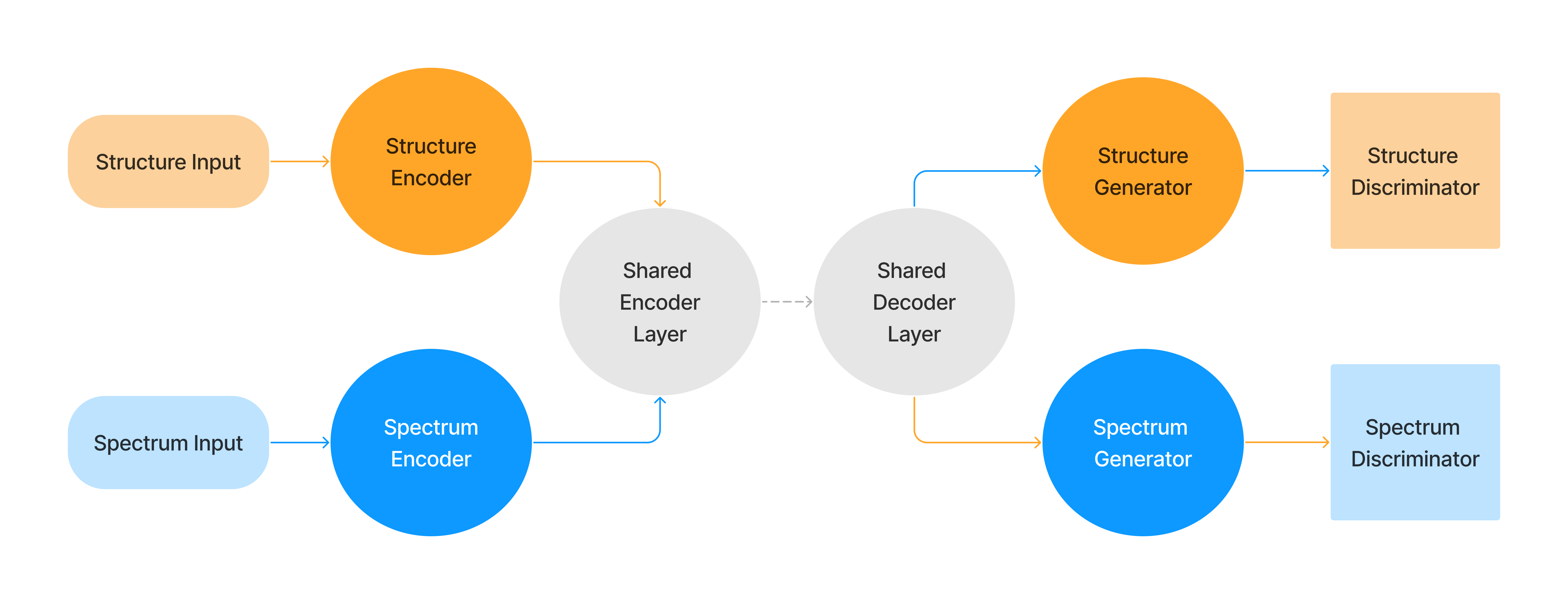
AEGAN-MLP

The AutoEncoding Generative Adversarial Network with Multi-Layer Perceptrons (AEGAN-MLP) model simultaneously trains both structure and spectra using two autoencoders (or generators) with shared parameters, along with two discriminators. The discriminators encourage better performance from the generators, while the generators attempt to fool the discriminators. This architecture allows separate pathways for each data type. The model can be used to either reconstruct the input data or predict the output data for structure or spectra without modifying the model. All components of the model are implemented as multilayer perceptron (MLP) networks. Except for the input and output dimensions, the size of the linear layers is currently fixed. The generative and discriminative parts of the model can use different loss functions, learning rates, and optimizers.

Training the AEGAN is achieved through alternating updates of the generative and discriminative components. The loss for the generative part is calculated as the sum of the scaled differences between model outputs and target outputs for both reconstructions and predictions of spectra and structure. Individual losses are scaled by the maximum value of the model output to compensate for differences in scaling between spectra and structure.

The discriminator attempts to predict whether the data is real (from the training set) or fake (produced by the generator). The total discriminator loss is the sum of the real and fake losses. The fake loss is calculated as the difference between the predicted labels for real and fake data generated by the generator. The real loss is calculated as the difference between the predicted labels for fake data and the true labels for real data.

Network Diagram:

Input file:

• type: aegan_mlp

• params:

  • hidden_size (int, 256): Size of the initial hidden layer.

  • num_hidden_layers_gen (int, 2): Number of hidden layers for the structure encoder and spectrum encoder in the generative part.

  • num_hidden_layers_shared (int, 2): Number of hidden layers for the shared encoder and shared decoder in the generative part.

  • num_hidden_layers_dis (int, 2): Number of hidden layers for the discriminative part.

  • activation (str, prelu): Activation function. Supported options: ReLU, Sigmoid, Tanh, PReLU, ELU, LeakyReLU, SELU, SiLU, GELU.

Example:

model:
  type: aegan_mlp
  params:
    hidden_size: 256
    activation: prelu
    num_hidden_layers_gen: 2
    num_hidden_layers_shared: 2
    num_hidden_layers_dis: 2
  weights:
    kernel: xavier_uniform
    bias: zeros
    seed: 2025

hyperparams:
    batch_size: 16
    epochs: 100
    seed: 2021
    lr: [0.01, 0.00001]     #[generative autoencoder, discriminator]
    optim_fn: [Adam, Adam]
    loss: [mse, bce]
    loss_reg: [None, None]
    loss_lambda: [0.001, 0.001]